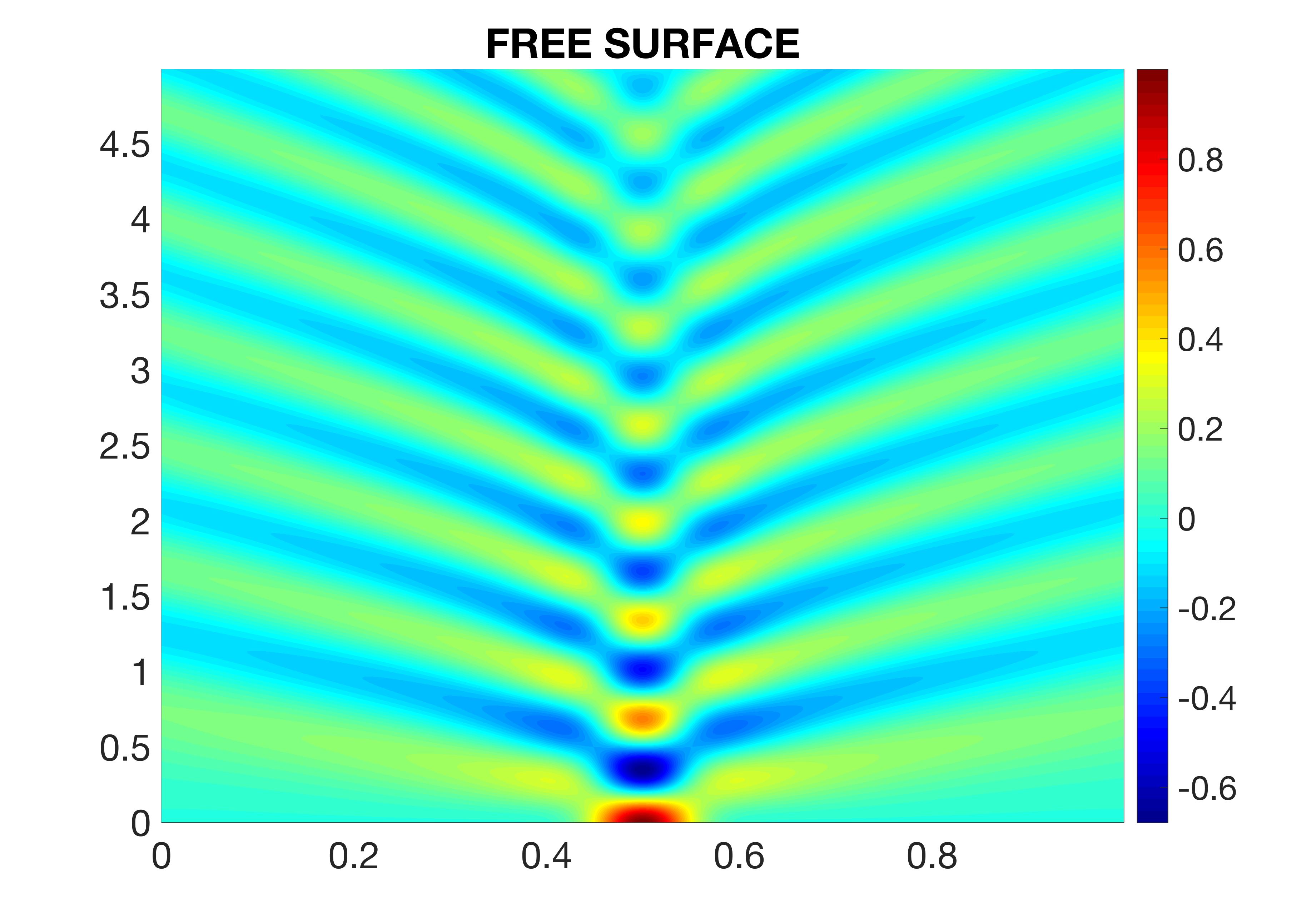
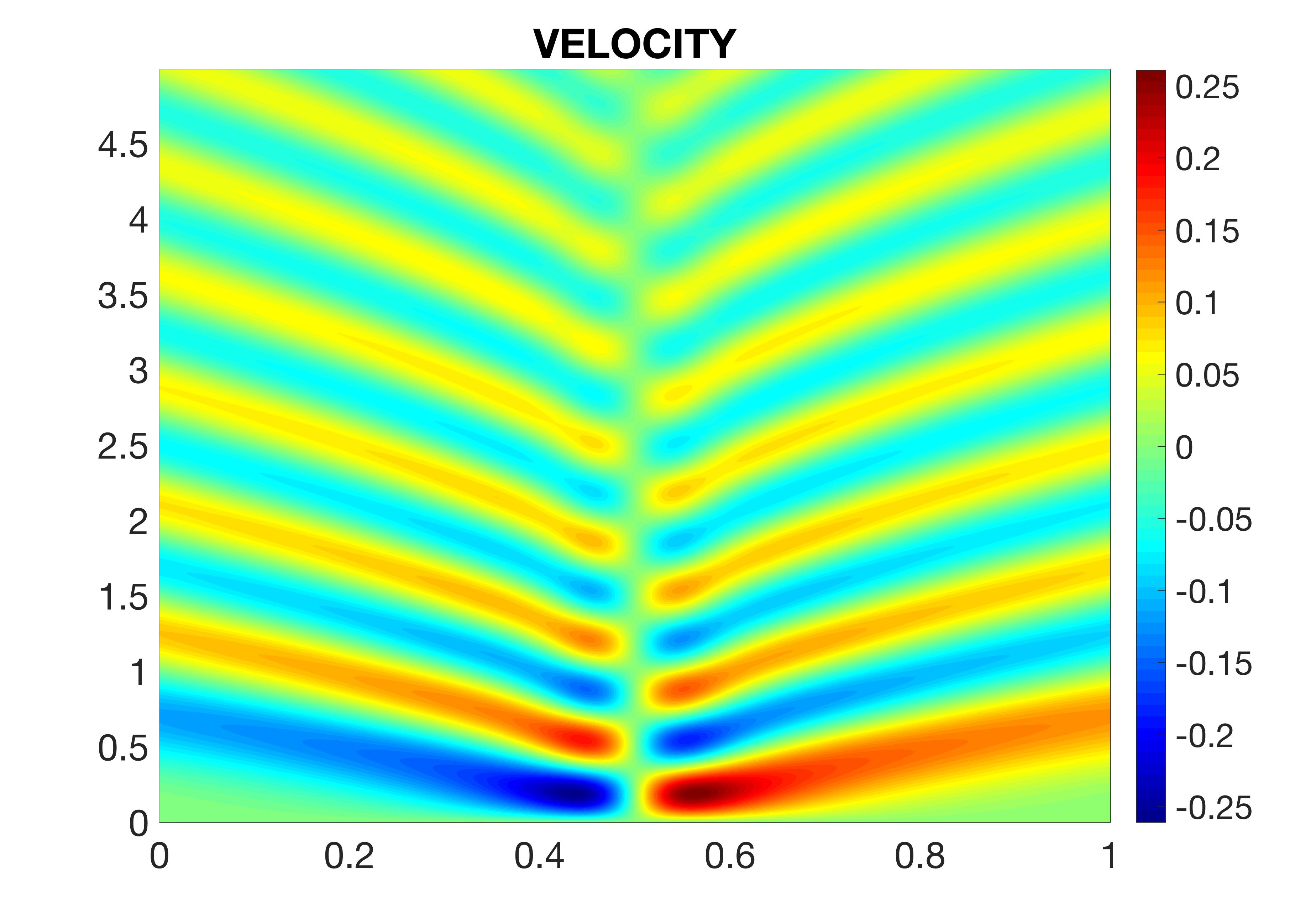
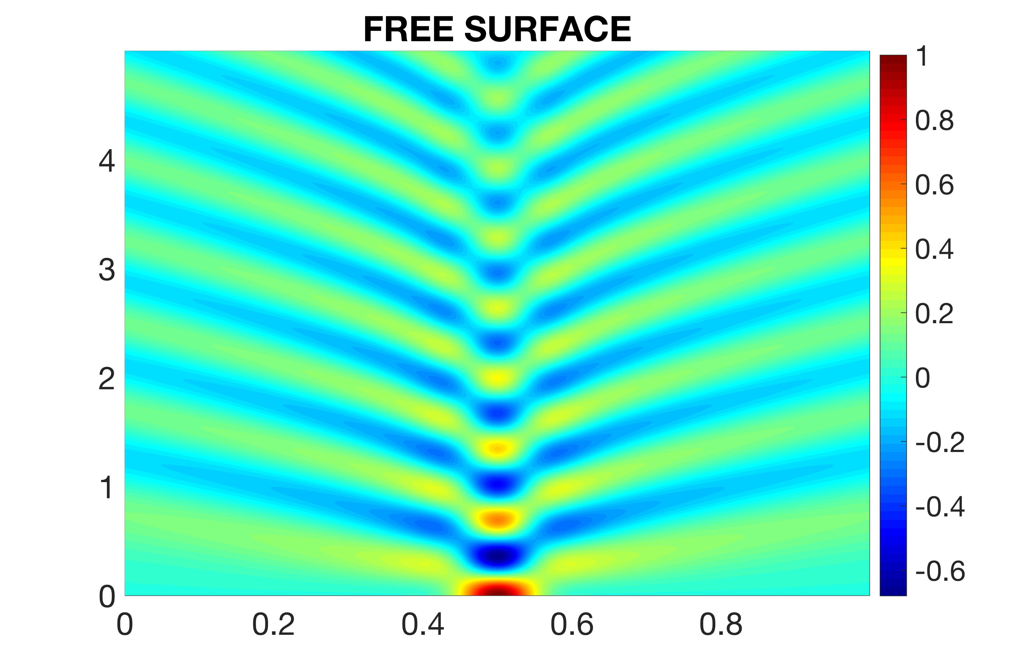
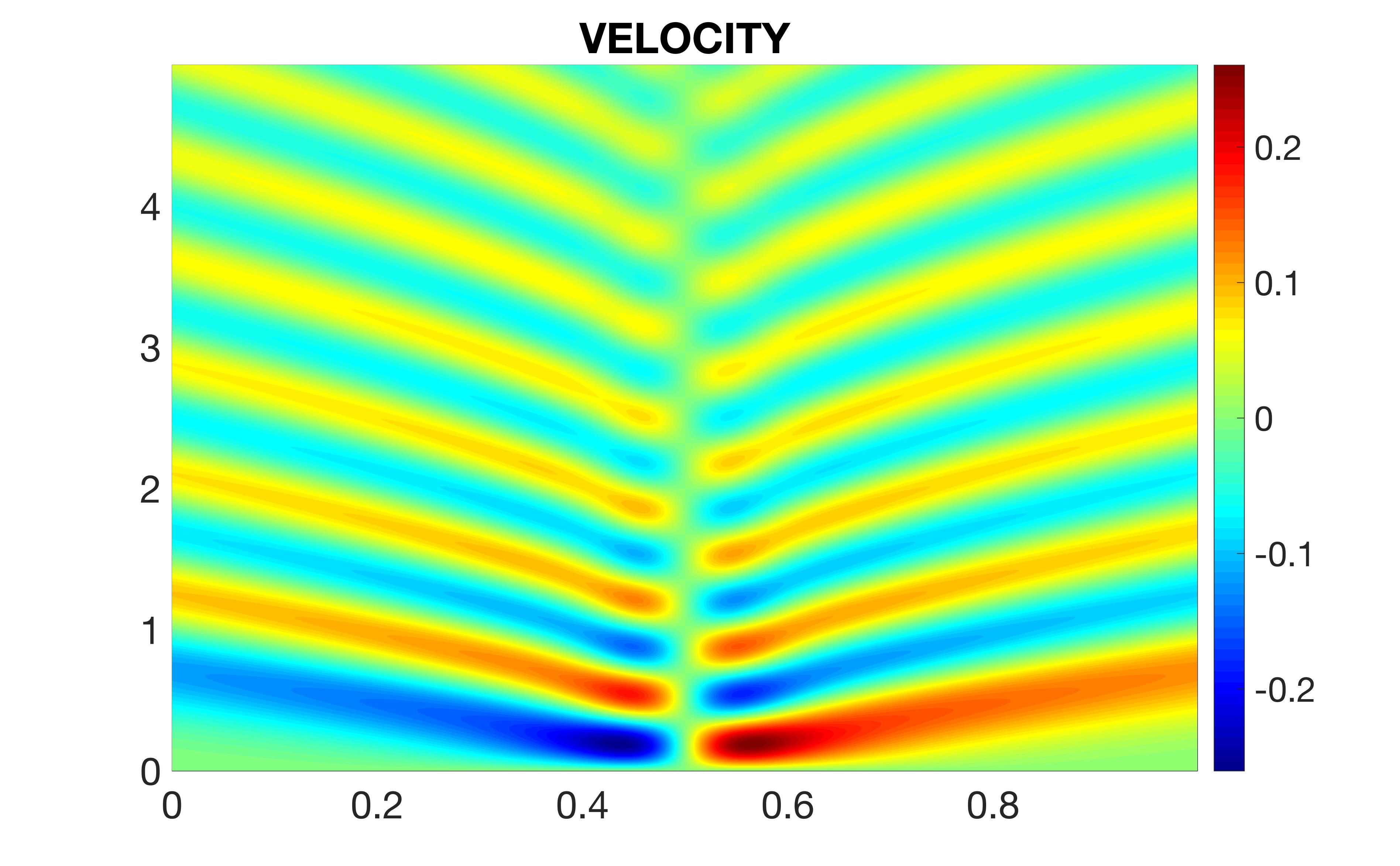
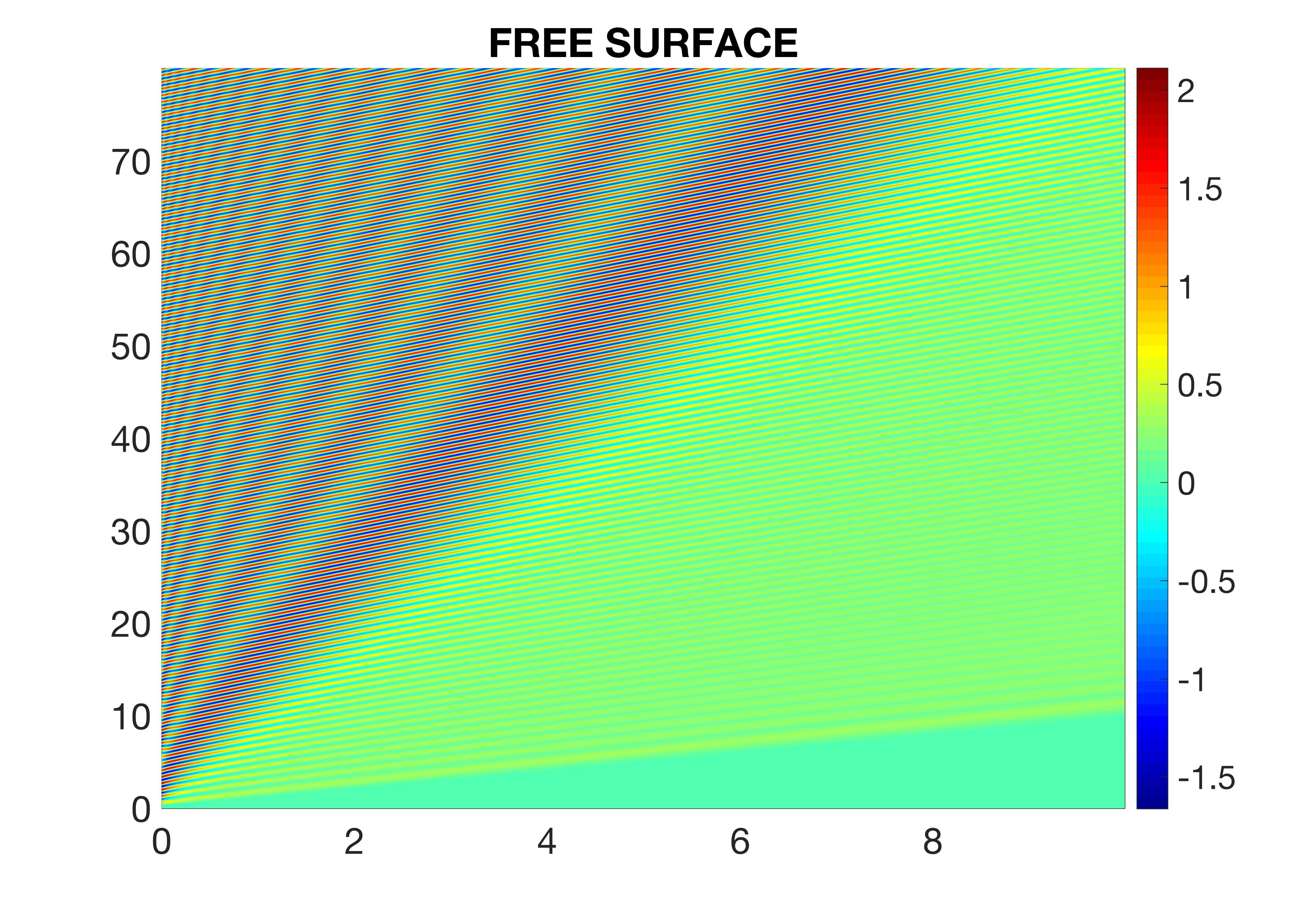
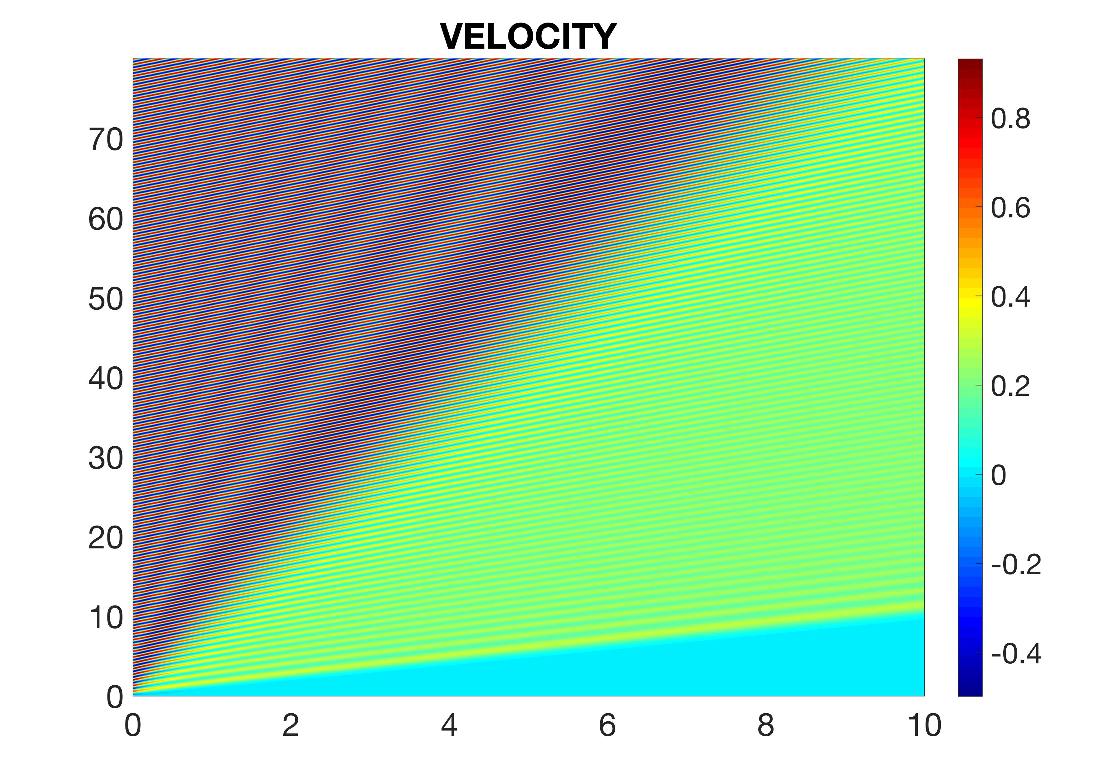
Transparent boundary conditions
Transparent boundary condition
Staggered grid scheme L = 1, N = 1025
Time step δt = 0.01
Dispersion parameter ε = 0.01
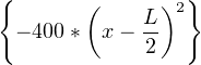
Gaussian initial data η(0,x) = 1 + exp
with zero velocity w(0,x) = 0.
Click on the image to restart the test animation