Chapter 4
State-transitions diagrams

Here is an example of state-transition diagram you can draw:

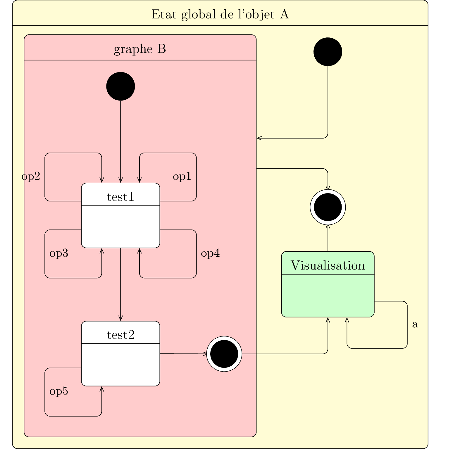
Now, we will see how to define parts of these diagrams, namely the ten sorts of state and the transitions.

4.1 To define a state

A "standard" state can be defined with the umlstate environment:

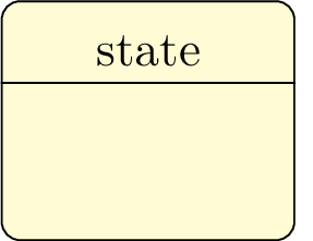
Both options x and y allows to place the state in the figure, or in another state. The default value is 0. The argument to give is the label of the state. The node representing the state has a default name, based on a global counter. For practical reasons, when you define a transition for instance, you can rename it with the name option.

You can also define the width of an empty state with the width option (8ex by default).

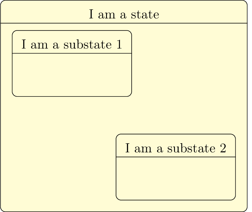
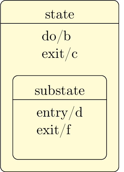
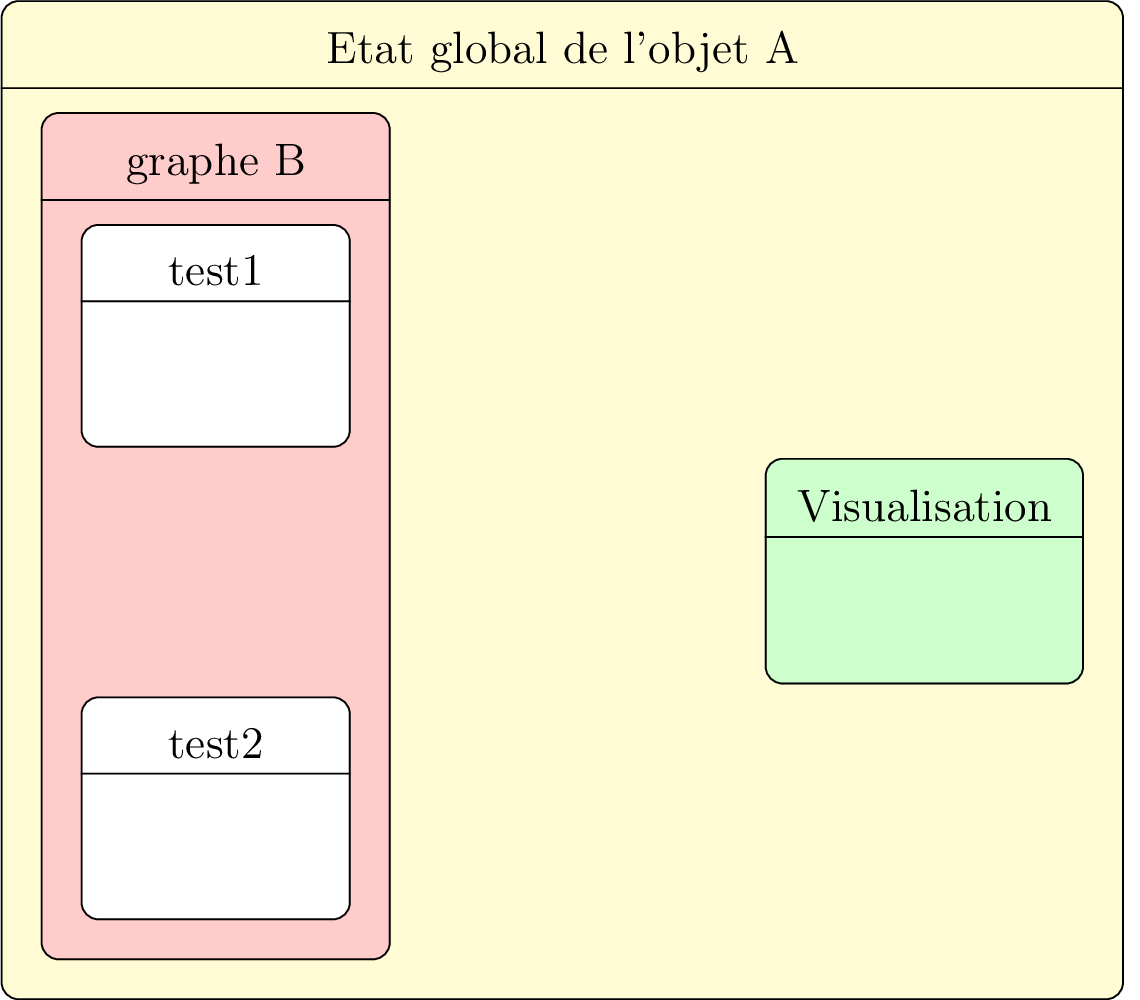
You can define a state in another state. Then, the coordinates of the sub-states are relative to the parent state:

If you want to define a state without detailing it, you can use the umlbasicstate command, that is an alias of the umlstate environment.

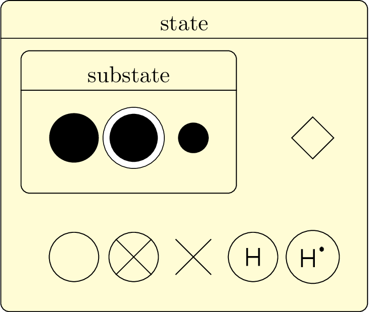
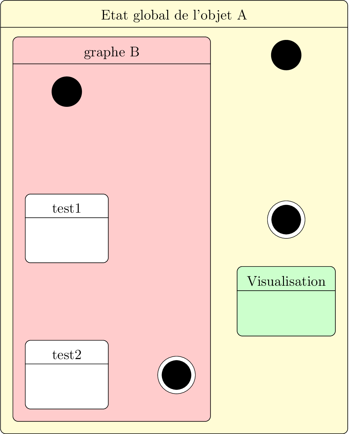
Let’s talk about the pseudo-states:

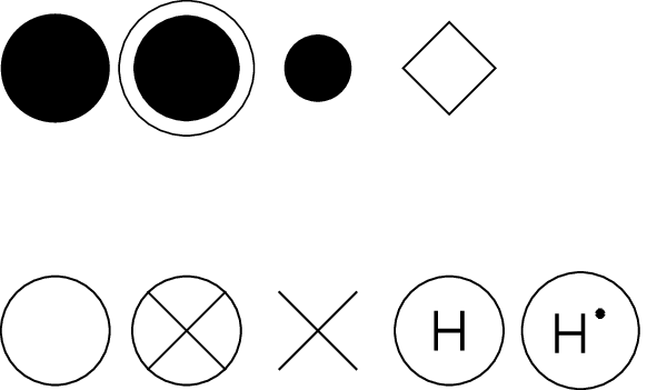
From left to right and top to bottom:

• An initial state is defined with the umlstateinitial command.
• A final state is defined with the umlstatefinal command.
• A join state is defined with the umlstatejoin command.
• A decision state is defined with the umlstatedecision command.
• An enter state is defined with the umlstateenter command.
• An exit state is defined with the umlstateexit command.
• An end state is defined with the umlstateend command.
• An history state is defined with the umlstatehistory command.
• A deep history state is defined with the umlstatedeephistory command.

These commands take several options: name, to rename the node, and width to set their size. You can use these commands in a umlstate environment:

You can also give actions on a state, through the entry, do and exit options:

4.2 To define a transition

Transitions are relations between states in a state-transition diagram. You can define them with the umltrans command, that is an alias of the umlrelation command. There are unidirectional transitions and recursive transitions.

4.2.1 To define a unidirectional transition

Thanks to the geometry option, usual aliases are available: umlHVtrans, umlVHtrans, umlVHVtrans and umlHVHtrans. Graphically, the use of these aliases are the most interesting, because corners are rounded.

Every option of the umlrelation command can be used with the umltrans command and its aliases.

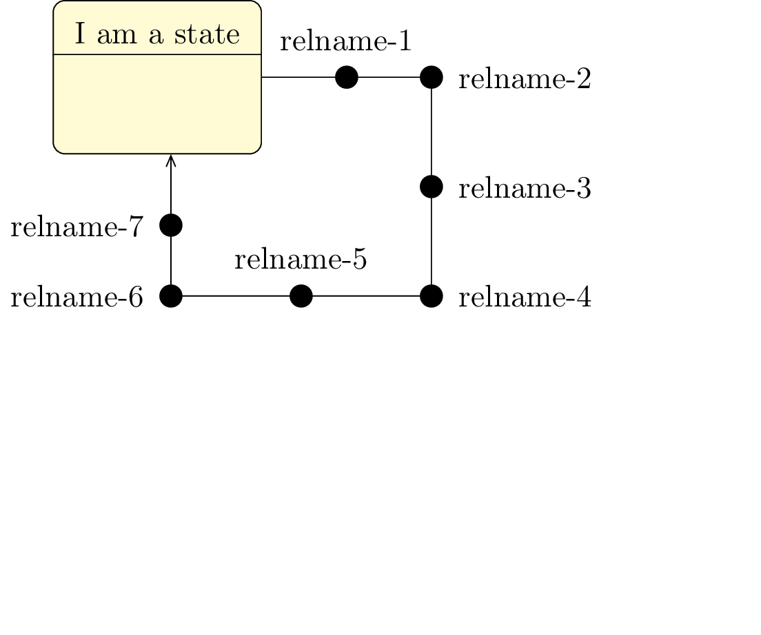
4.2.2 To define a recursive transition

Recursive transitions are graphically the most difficult to manage, because their shape is a rounded rectangle, contrary to recursive relations in a class diagram. Conceptually, it is as if the geometry option has the value -|- or |-|, that is to say arrows composed of several segments.

The recursive direction option is fundamental. Indeed, giving values of start angle and end angle is not enough to determine the start direction and the end direction of the recursive arrow, because it does not define the normal direction. Then, we have to precise it. There are 2 cases:

• The arrow can be composed of 3 segments. In this case, usable nodes are shown as follows:

  

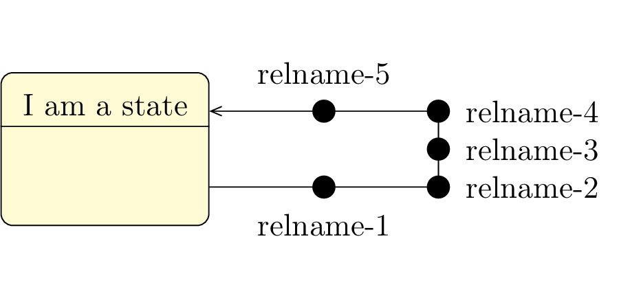
• The arrow can be composed of 4 segments. In this case, usable nodes are shown as follows:

  

4.2.3 To define a transition between sub states

When you want to define transitions between sub-states, transitions are drawn inside the parent state.Then, you have to define them inside the umlstate environment. Let’s compare the two following examples:

4.3 Advanced features for positioning

umlstate and the 9 pseudo-state commands can accept every option key defined for nodes in TikZ . In this section, you will see how some of them can be used for advanced features.

4.3.1 Horizontal and vertical alignment

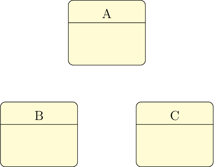
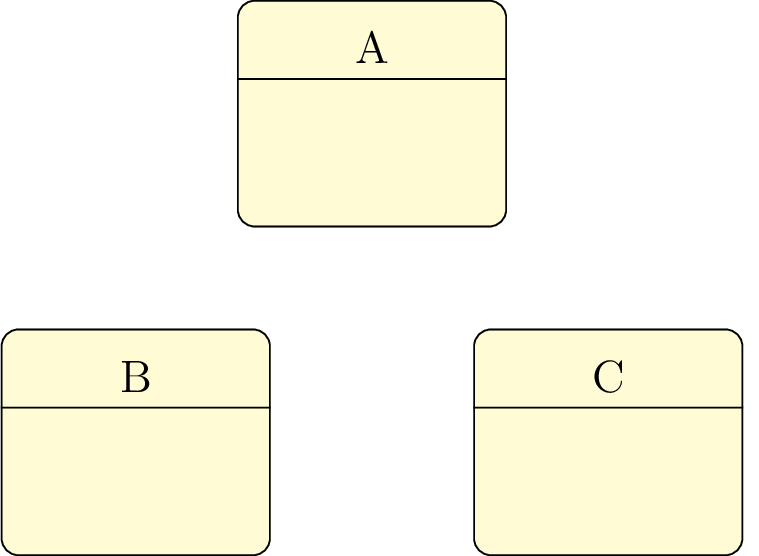
In a state-transition diagram, states have different width and height. For a graphical purpose, you may want to align them horizontally or vertically. Let’s take the following example:

The y coordinate defines the center of the state node. It will be better in this example to have states B and C top-aligned. A solution is to define manually the y value for C, but it is not very convenient. You may prefer use the anchor option. If you specify anchor=north, the y coordinate will define the top center anchor of the node, instead of the center. You may take a look at the differences between both codes.

In a similar way, you may use anchor=east to right align states, anchor=west to left align states or anchor=south to bottom align states.

4.3.2 Relative positioning

Using the x-y coordinate system may be very hard in big diagrams, when you have to change position of elements in order to fit the diagram to the page. Relative positioning may be useful in this case, namely advanced syntax of options above, left, below, right, above left, below left, below right and above right provided by the TikZ library positioning.

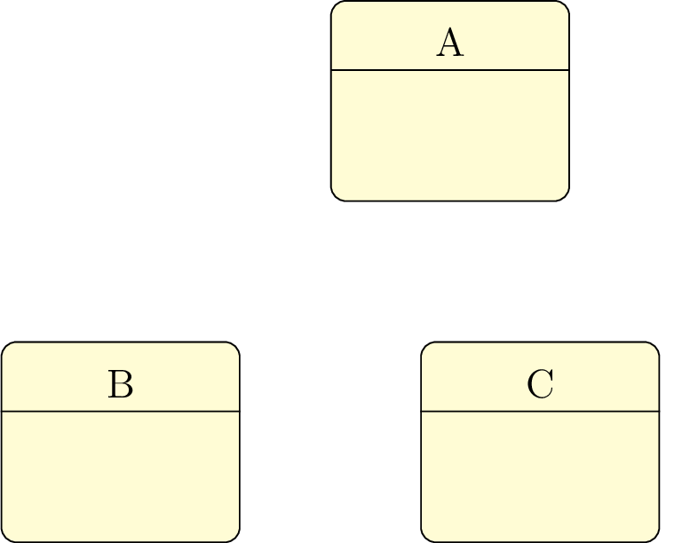
Let’s take the previous example, you can define B by its cordinates (-2,-2) or by saying that B is 2cm below and 2cm left of A. You can also define C by saying it is 4cm right of B. Notice that because of the top alignment of B and C, the latter is defined 4cm right of B.north.

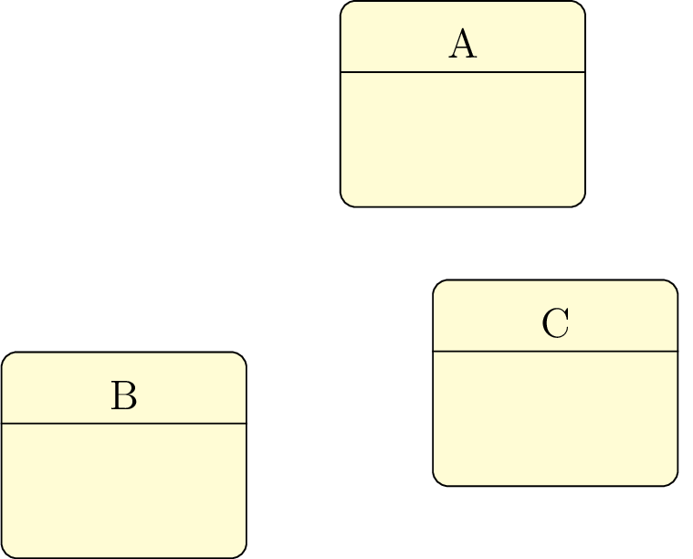
The behavior is not the one expected. It is because definition of a state node is complex. Instead of B, you may use here B-body.

4.4 To change preferences

With the tikzumlset command, you can change default colors for states and transitions:

text:

allows to set default text color (=black by default),

draw:

allows to set the default edge color and the default color of initial, final and join states (=black by default),

fill state:

allows to set the default background color of a state (=yellow!20 by default),

font:

allows to set the default font style (=\small by default).

state join width

allows to set the default with of a state join (=3ex by default),

state decision width:

allows to set the default width of a state decision (=3ex by default),

state initial width:

allows to set the default width of a state initial (=5ex by default),

state final width:

allows to set the default width of a state final (=5.5ex by default),

state enter width:

allows to set the default width of a state enter (=5ex by default),

state exit width:

allows to set the default width of a state exit (=5ex by default),

state end width:

allows to set the default wdith of a state end (=5ex by default),

state history width:

allows to set the default width of a state history (=5ex by default),

state deep history width:

allows to set the default width of a state deep-history (=5ex by default),

state width:

allows to set the default width of a state (=8ex by default)

You can also use the text, draw and fill options on a particular element, in order to change its colors, as shown in the introduction example.

4.5 Examples

4.5.1 Example from introduction, step by step

Definition of basic states

Definition of specific states

Definition of transitions