Overview of the BiNoPe-HJ project

The HJB Solver aims at computing approximate solution to Hamilton-Jacobi equations of the following form :

u + H (x,∇u ) = 0, x ∈ Ω

{ ∂u+ H (x,∇u) = 0, t ∈ (0,T), x ∈ Ω ∂ut(0,x) = u(x), x ∈ Ω 0

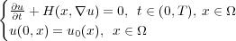together with some boundary conditions on the boundary ∂Ω of Ω, and where typically :

H(x,∇u) ≡ max_α(-f(x,α).∇u - ℓ(x,α))
Ω : "box" domain of ℝ^d with d ≥ 2
f : ℝ⁺ × ℝ^d × ℝ^m → ℝ^d : dynamics of the system
ℓ : ℝ⁺ × ℝ^d × ℝ^m → ℝ : distributed cost function
U : commands set and m := |U| number of commands (if they are discretized).

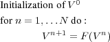
1 Architecture

The d-dimensional solver is implemented with mainly two schemes : the Semi-Lagrangian scheme and the Finite Difference scheme. The general structure of is the following :

0 Initialization ofV forn = 1,...N do : V n+1 = F (V n)

Also, sequentials version of the Fast Marching Method have been implemented in dimension d, adapted to solving the eikonal equation of the form c(x,u(x))∥∇u(x)∥ = 1 for x ∈ Ω, with u(x) = 0 for x ∈ Ω₀ ⊂ Ω.

2 Numerical methods

Semi Lagrangien Scheme.

It is implemented with P1 interpolations of the caracteristics which are computed using EDO discretization method such as Euler (RK1), Heun or midpoint rule (RK2).

Finite Differences Scheme.

first order Lax-Friedrichs scheme and second order ENO2 (Essentially Non Oscillatory) scheme are implemented, and are coupled with Runge-Kutta methods on order 1, 2 or 3 in time.

Fast Marching Method (FMM)

for Eikonal equations, 3 different cases :

classical FMM for problems with a constant sign, time-independent velocity : c(x)∥∇u(x)∥ = 1 and with c(x) > 0
time-dependent FMM for problems with constant sign, time-dependent velocity c = c(x,t) and with c(x,t) ≥ 0
Generalized FMM for problems with a changing-sign, time-dependant velocity : c(x,u(x)))∥∇u(x)∥ = 1 and with c(x) > 0